Deep Dive: DC Transport and Emission¶

DC Transport Theory¶

When a DC electric field is applied along the quantum wire, carriers drift in momentum space. The drift velocity is:

\[ v_{drift} = \frac{\sum_k \frac{\hbar k}{m} \cdot f(k)}{\sum_k f(k)} \]

where \(f(k)\) is the carrier distribution and \(m\) is the effective mass. The DC transport module shifts the distribution in momentum space by \(\Delta k = eE_{dc} \Delta t / \hbar\) at each time step.

Phonon-Assisted Drift¶

Phonon scattering opposes the drift by scattering carriers back toward equilibrium. The steady-state drift velocity results from the balance between the DC field acceleration and phonon friction.

Current Density¶

The current density along the wire is:

\[ J = \frac{e}{L} \sum_k \left[ \frac{\hbar k}{m_e} n_e(k) - \frac{\hbar k}{m_h} n_h(k) \right] \]

Spontaneous Emission Theory¶

Electron-hole pairs recombine radiatively, emitting photons. The spontaneous emission rate depends on the carrier overlap and the photon density of states:

\[ R_{sp}(k) = \frac{3 |d_{cv}|^2}{\epsilon_0 \sqrt{\epsilon_r}} \cdot n_e(k) \cdot n_h(k) \cdot \rho_{photon}(E_k) \]

Photoluminescence Spectrum¶

The PL spectrum is the frequency-resolved emission:

\[ PL(\hbar\omega) = R_{scale} \sum_k n_e(k) \, n_h(k) \, \hbar\omega \, \rho_0(\hbar\omega) \, L(\hbar\omega - E_k, \gamma_{eh}) \, e^{-|\hbar\omega - E_k| / k_B T} \]

where \(L\) is a Lorentzian lineshape and \(\rho_0\) is the photon density of states.

Initialize and Inspect¶

import os
import numpy as np
import matplotlib.pyplot as plt
from scipy.constants import hbar as hbar_SI, k as kB_SI, e as e0_SI

from pulsesuite.PSTD3D.SBEs import InitializeSBE
from pulsesuite.PSTD3D import SBEs as SBEs_module
from pulsesuite.PSTD3D import dcfield, emission
from pulsesuite.PSTD3D.typespace import GetKArray, GetSpaceArray

# Ensure output directories exist
for d in ['dataQW/Wire/C', 'dataQW/Wire/D', 'dataQW/Wire/Ee',
          'dataQW/Wire/Eh', 'dataQW/Wire/P', 'dataQW/Wire/Win',
          'dataQW/Wire/Wout', 'dataQW/Wire/Xqw', 'dataQW/Wire/info',
          'dataQW/Wire/ne', 'dataQW/Wire/nh', 'output']:
    os.makedirs(d, exist_ok=True)

Nr = 50
drr = 10e-9
rr = GetSpaceArray(Nr, (Nr - 1) * drr)
qrr = GetKArray(Nr, Nr * drr)

InitializeSBE(qrr, rr, 0.0, 1e7, 800e-9, 2, True)
solver = SBEs_module._default_solver

print(f"DCTrans enabled: {solver.DCTrans}")
print(f"Recomb enabled: {solver.Recomb}")
print(f"DC field: {solver.Edc} V/m")
print(f"Electron mass: {solver.me / 9.109e-31:.4f} m0")
print(f"Hole mass: {solver.mh / 9.109e-31:.4f} m0")

dcv / e0 = 3.3538811268940077e-10
alphae = 303090660.34386384, alphah = 768475083.4742767
1/qc = 2.3003106022655407e-09, sqrt(2) / sqrt(alphae² + alphah²) = 1.7119449377756965e-09
ehint = 0.8262109841666643
Wire Radius = 2.3003106022655407e-09
Wire sqrt(area) = 3.8950888292173374e-09
Wire Thickness = 5e-09

Calculating Coulomb Arrays
  Progress: 0/230 (0.0%)
Vint: Using JIT-compiled version
  Progress: 10/230 (4.3%)
  Progress: 20/230 (8.7%)
  Progress: 30/230 (13.0%)
  Progress: 40/230 (17.4%)
  Progress: 50/230 (21.7%)
  Progress: 60/230 (26.1%)
  Progress: 70/230 (30.4%)
  Progress: 80/230 (34.8%)
  Progress: 90/230 (39.1%)
  Progress: 100/230 (43.5%)
  Progress: 110/230 (47.8%)
  Progress: 120/230 (52.2%)
  Progress: 130/230 (56.5%)
  Progress: 140/230 (60.9%)
  Progress: 150/230 (65.2%)
  Progress: 160/230 (69.6%)
  Progress: 170/230 (73.9%)
  Progress: 180/230 (78.3%)
  Progress: 190/230 (82.6%)
  Progress: 200/230 (87.0%)
  Progress: 210/230 (91.3%)
  Progress: 220/230 (95.7%)
Finished Calculating Unscreened Coulomb Arrays

Quantum Wire Linear Chi = (-0.13219666733079763+0.14243061062572296j)

InitializeSBE?
DCTrans enabled: True
Recomb enabled: True
DC field: 0.0 V/m
Electron mass: 0.0700 m0
Hole mass: 0.4500 m0

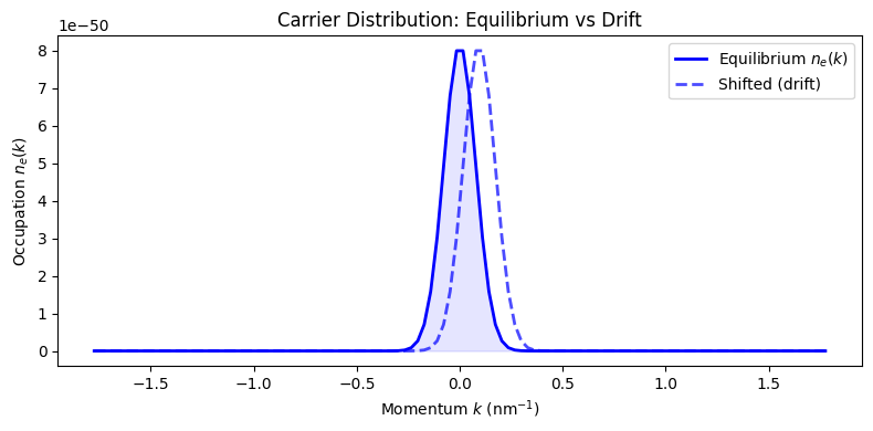
Drift Velocity Calculation¶

The CalcVD function computes the drift velocity from a carrier distribution. With the initial thermal distribution and zero DC field, the drift velocity is zero (symmetric distribution). We can artificially shift the distribution to demonstrate the calculation.

eV = 1.6e-19
k_nm = solver.kr * 1e-9

# Initial thermal distribution (symmetric -> zero drift)
ne = np.real(np.diag(solver.CC2[:, :, 0]))
nh = np.real(np.diag(solver.DD2[:, :, 0]))

v_e = dcfield.CalcVD(solver.kr, solver.me, ne.astype(complex))
v_h = dcfield.CalcVD(solver.kr, solver.mh, nh.astype(complex))

print(f"Initial drift velocity (electrons): {v_e:.2e} m/s (should be ~0)")
print(f"Initial drift velocity (holes):     {v_h:.2e} m/s (should be ~0)")

# Demonstrate: shift distribution to simulate drift
dk_shift = 3  # shift by 3 grid points
ne_shifted = np.roll(ne, dk_shift)

v_e_shifted = dcfield.CalcVD(solver.kr, solver.me, ne_shifted.astype(complex))
print(f"\nAfter shifting {dk_shift} grid points:")
print(f"Drift velocity: {v_e_shifted:.2e} m/s")
print(f"Corresponding to drift energy: {0.5 * solver.me * v_e_shifted**2 / eV * 1e3:.2f} meV")

Initial drift velocity (electrons): 2.32e-103 m/s (should be ~0)
Initial drift velocity (holes):     3.60e-104 m/s (should be ~0)

After shifting 3 grid points:
Drift velocity: 1.56e+05 m/s
Corresponding to drift energy: 4.84 meV

fig, ax = plt.subplots(figsize=(8, 4))

ax.plot(k_nm, ne, 'b-', linewidth=2, label='Equilibrium $n_e(k)$')
ax.plot(k_nm, ne_shifted, 'b--', linewidth=2, alpha=0.7, label='Shifted (drift)')
ax.fill_between(k_nm, 0, ne, alpha=0.1, color='blue')

ax.set_xlabel('Momentum $k$ (nm$^{-1}$)')
ax.set_ylabel('Occupation $n_e(k)$')
ax.set_title('Carrier Distribution: Equilibrium vs Drift')
ax.legend()
plt.tight_layout()
plt.show()

../_images/dbb1733ce6460fb2fd3ebfa262714849776d5672465490611a14431a7240e8ed.png

Spontaneous Emission¶

The emission module computes radiative recombination rates using the real carrier distributions and Coulomb-renormalized energies from initialization.

print(f"Emission scale factor: {emission._RScale:.3e}")
print(f"Temperature: {emission._Temp} K")
print(f"Energy grid for emission: {len(emission._HOmega)} points")
print(f"Energy range: {emission._HOmega[0]/eV*1e3:.1f} to {emission._HOmega[-1]/eV*1e3:.1f} meV")

Emission scale factor: 2.214e-46
Temperature: 77.0 K
Energy grid for emission: 887 points
Energy range: 0.0 to 29.2 meV

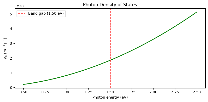
Photon Density of States¶

The photon density of states \(\rho_0(\hbar\omega) = (\hbar\omega)^2 / (\pi^2 \hbar^3 c^3)\) determines which photon energies have the most available modes for emission.

hw_range = np.linspace(0.5 * eV, 2.5 * eV, 200)
rho0_vals = emission.rho0(hw_range)

fig, ax = plt.subplots(figsize=(8, 4))
ax.plot(hw_range / eV, rho0_vals, 'g-', linewidth=2)
ax.axvline(solver.gap / eV, color='red', linestyle='--', alpha=0.7,
           label=f'Band gap ({solver.gap/eV:.2f} eV)')
ax.set_xlabel('Photon energy (eV)')
ax.set_ylabel('$\\rho_0$ (m$^{-3}$ J$^{-1}$)')
ax.set_title('Photon Density of States')
ax.legend()
plt.tight_layout()
plt.show()

../_images/b9c0a3722d6a0282759ec7a0253e5e4122a2bbc92b670c78946efa18a73b6750.png

References¶

J. R. Gulley and D. Huang, Opt. Express 27, 17154-17185 (2019). – DC transport and emission within the self-consistent SBE framework.
J. R. Gulley, R. Cooper, and E. Winchester, “Mobility and conductivity of laser-generated e-h plasmas in direct-gap nanowires,” Photonics Nanostructures: Fundam. Appl. 59, 101259 (2024).