Deep Dive: Coulomb Interactions

Theory

The Coulomb module calculates carrier-carrier interactions in the quantum wire. These enter the SBE Hamiltonians as screened interaction matrices.

Coulomb Interaction Potential

The interaction between carriers confined in a quantum wire is:

\[ V(k, q) = \frac{e^2}{2\pi \epsilon_0 \epsilon_r L} \int dy_1 \, dy_2 \; |\phi_e(y_1)|^2 |\phi_h(y_2)|^2 \, K_0(|k-q| \, r) \]

where \(K_0\) is the modified Bessel function of the second kind, \(r = \sqrt{(y_1-y_2)^2 + \Delta_0^2}\) accounts for the wire thickness, and \(\phi_{e/h}\) are the confinement wavefunctions.

The Bessel function \(K_0(x) \sim -\ln(x/2)\) for small \(x\), giving the characteristic logarithmic divergence of the 1D Coulomb potential at \(k=q\) (same momentum).

Energy Renormalization

Many-body Coulomb interactions renormalize the single-particle energies:

Band Gap Renormalization (BGR):

\[ \Delta E_{gap} = -\sum_k [n_e(k) V_{ee}(k,k) + n_h(k) V_{hh}(k,k)] \]

Electron/Hole Energy Renormalization:

\[ \Delta E_e(k) = \sum_{k'} n_e(k') [V_{ee}(k,k) - V_{ee}(k,k')] \]

Screening

Free carriers screen the bare Coulomb interaction:

\[ V_{screened}(q) = \frac{V_{bare}(q)}{\epsilon(q)} \]

where \(\epsilon(q)\) is the static dielectric function computed from the 1D Lindhard susceptibility.

---

Initialize and Inspect

We call InitializeSBE which internally calls InitializeCoulomb with real material parameters. Then we access the computed Coulomb arrays.

import os
import numpy as np
import matplotlib.pyplot as plt

from pulsesuite.PSTD3D.SBEs import InitializeSBE
from pulsesuite.PSTD3D import SBEs as SBEs_module
from pulsesuite.PSTD3D import coulomb
from pulsesuite.PSTD3D.typespace import GetKArray, GetSpaceArray

# Ensure output directories exist
for d in ['dataQW/Wire/C', 'dataQW/Wire/D', 'dataQW/Wire/Ee',
          'dataQW/Wire/Eh', 'dataQW/Wire/P', 'dataQW/Wire/Win',
          'dataQW/Wire/Wout', 'dataQW/Wire/Xqw', 'dataQW/Wire/info',
          'dataQW/Wire/ne', 'dataQW/Wire/nh', 'output']:
    os.makedirs(d, exist_ok=True)

Nr = 50
drr = 10e-9
rr = GetSpaceArray(Nr, (Nr - 1) * drr)
qrr = GetKArray(Nr, Nr * drr)

InitializeSBE(qrr, rr, 0.0, 1e7, 800e-9, 2, True)
solver = SBEs_module._default_solver
cm = coulomb._instance  # CoulombModule singleton

print(f"Coulomb module initialized for Nk={solver.Nk} momentum points")
print(f"Unscreened Coulomb matrices: Veh0 {cm.Veh0.shape}, Vee0 {cm.Vee0.shape}, Vhh0 {cm.Vhh0.shape}")

dcv / e0 = 3.3538811268940077e-10
alphae = 303090660.34386384, alphah = 768475083.4742767
1/qc = 2.3003106022655407e-09, sqrt(2) / sqrt(alphae² + alphah²) = 1.7119449377756965e-09
ehint = 0.8262109841666643
Wire Radius = 2.3003106022655407e-09
Wire sqrt(area) = 3.8950888292173374e-09
Wire Thickness = 5e-09

Calculating Coulomb Arrays
  Progress: 0/230 (0.0%)
Vint: Using JIT-compiled version
  Progress: 10/230 (4.3%)
  Progress: 20/230 (8.7%)
  Progress: 30/230 (13.0%)
  Progress: 40/230 (17.4%)
  Progress: 50/230 (21.7%)
  Progress: 60/230 (26.1%)
  Progress: 70/230 (30.4%)
  Progress: 80/230 (34.8%)
  Progress: 90/230 (39.1%)
  Progress: 100/230 (43.5%)
  Progress: 110/230 (47.8%)
  Progress: 120/230 (52.2%)
  Progress: 130/230 (56.5%)
  Progress: 140/230 (60.9%)
  Progress: 150/230 (65.2%)
  Progress: 160/230 (69.6%)
  Progress: 170/230 (73.9%)
  Progress: 180/230 (78.3%)
  Progress: 190/230 (82.6%)
  Progress: 200/230 (87.0%)
  Progress: 210/230 (91.3%)
  Progress: 220/230 (95.7%)
Finished Calculating Unscreened Coulomb Arrays

Quantum Wire Linear Chi = (-0.13219666733079763+0.14243061062572296j)

InitializeSBE?
Coulomb module initialized for Nk=114 momentum points
Unscreened Coulomb matrices: Veh0 (114, 114), Vee0 (114, 114), Vhh0 (114, 114)

Unscreened Coulomb Matrices

The three interaction matrices \(V_{eh}\), \(V_{ee}\), \(V_{hh}\) in momentum space. The diagonal (\(k=k'\)) is strongest because carriers at the same momentum have maximum spatial overlap. The off-diagonal elements mediate scattering.

fig, axes = plt.subplots(1, 3, figsize=(14, 4))

eV = 1.6e-19
k_nm = solver.kr * 1e-9

for ax, V, title in zip(axes,
                         [cm.Veh0, cm.Vee0, cm.Vhh0],
                         ['$V_{eh}$ (e-h)', '$V_{ee}$ (e-e)', '$V_{hh}$ (h-h)']):
    im = ax.pcolormesh(k_nm, k_nm, np.real(V) / eV,
                        shading='auto', cmap='RdBu_r')
    ax.set_xlabel('$k$ (nm$^{-1}$)')
    ax.set_ylabel("$k'$ (nm$^{-1}$)")
    ax.set_title(title)
    ax.set_aspect('equal')
    plt.colorbar(im, ax=ax, label='eV')

plt.suptitle('Unscreened Coulomb Interaction Matrices', y=1.02)
plt.tight_layout()
plt.show()

print(f"Veh diagonal range: {np.real(cm.Veh0).diagonal().min()/eV:.4f} to "
      f"{np.real(cm.Veh0).diagonal().max()/eV:.4f} eV")
print(f"Vee diagonal range: {np.real(cm.Vee0).diagonal().min()/eV:.4f} to "
      f"{np.real(cm.Vee0).diagonal().max()/eV:.4f} eV")

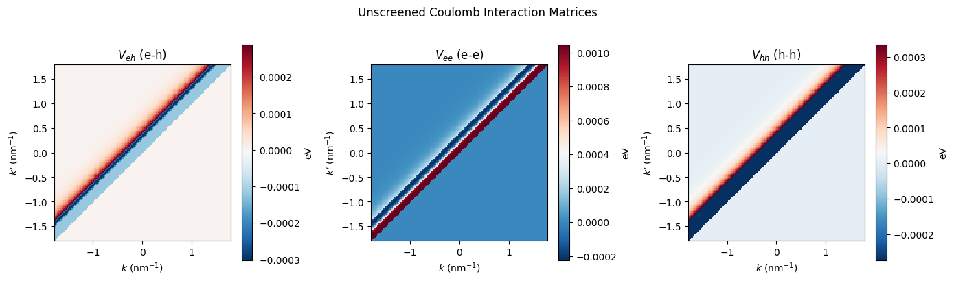
Veh diagonal range: -0.0001 to -0.0001 eV
Vee diagonal range: 0.0010 to 0.0010 eV

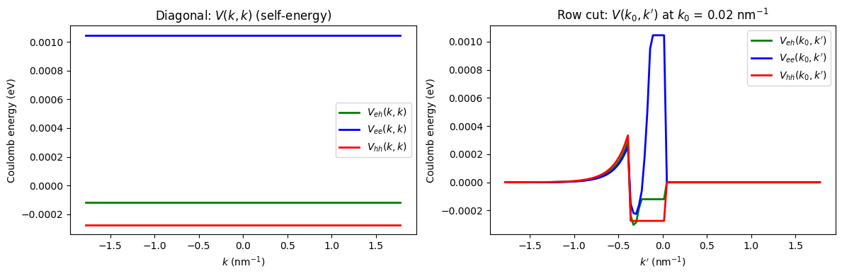
Momentum-Space Cuts

A cut along the diagonal (\(k=k'\)) shows the self-energy contribution. A cut at fixed \(k\) shows how the interaction decays with momentum transfer.

fig, (ax1, ax2) = plt.subplots(1, 2, figsize=(12, 4))

# Diagonal cut: V(k, k)
ax1.plot(k_nm, np.real(cm.Veh0).diagonal() / eV, 'g-', linewidth=2, label='$V_{eh}(k,k)$')
ax1.plot(k_nm, np.real(cm.Vee0).diagonal() / eV, 'b-', linewidth=2, label='$V_{ee}(k,k)$')
ax1.plot(k_nm, np.real(cm.Vhh0).diagonal() / eV, 'r-', linewidth=2, label='$V_{hh}(k,k)$')
ax1.set_xlabel('$k$ (nm$^{-1}$)')
ax1.set_ylabel('Coulomb energy (eV)')
ax1.set_title('Diagonal: $V(k, k)$ (self-energy)')
ax1.legend()

# Off-diagonal cut at k=0 (midpoint of grid)
mid_k = solver.Nk // 2
ax2.plot(k_nm, np.real(cm.Veh0[mid_k, :]) / eV, 'g-', linewidth=2, label='$V_{eh}(k_0, k\')$')
ax2.plot(k_nm, np.real(cm.Vee0[mid_k, :]) / eV, 'b-', linewidth=2, label='$V_{ee}(k_0, k\')$')
ax2.plot(k_nm, np.real(cm.Vhh0[mid_k, :]) / eV, 'r-', linewidth=2, label='$V_{hh}(k_0, k\')$')
ax2.set_xlabel("$k'$ (nm$^{-1}$)")
ax2.set_ylabel('Coulomb energy (eV)')
ax2.set_title(f'Row cut: $V(k_0, k\')$ at $k_0$ = {k_nm[mid_k]:.2f} nm$^{{-1}}$')
ax2.legend()

plt.tight_layout()
plt.show()

Many-Body Broadening Arrays

The matrices \(C_{eh}\), \(C_{ee}\), \(C_{hh}\) control the energy-conservation broadening in many-body collision integrals. They determine which scattering channels are energetically allowed.

fig, axes = plt.subplots(1, 3, figsize=(14, 4))

for ax, C, title in zip(axes,
                         [cm.Ceh, cm.Cee, cm.Chh],
                         ['$C_{eh}$', '$C_{ee}$', '$C_{hh}$']):
    im = ax.pcolormesh(k_nm, k_nm, np.real(C),
                        shading='auto', cmap='viridis')
    ax.set_xlabel('$k$ (nm$^{-1}$)')
    ax.set_ylabel("$k'$ (nm$^{-1}$)")
    ax.set_title(title)
    ax.set_aspect('equal')
    plt.colorbar(im, ax=ax)

plt.suptitle('Many-Body Broadening Matrices', y=1.02)
plt.tight_layout()
plt.show()

print(f"Ceh range: {np.real(cm.Ceh).min():.3e} to {np.real(cm.Ceh).max():.3e}")
print(f"Cee range: {np.real(cm.Cee).min():.3e} to {np.real(cm.Cee).max():.3e}")

---------------------------------------------------------------------------
TypeError                                 Traceback (most recent call last)
Cell In[4], line 6
      1 fig, axes = plt.subplots(1, 3, figsize=(14, 4))
      3 for ax, C, title in zip(axes,
      4                          [cm.Ceh, cm.Cee, cm.Chh],
      5                          ['$C_{eh}$', '$C_{ee}$', '$C_{hh}$']):
----> 6     im = ax.pcolormesh(k_nm, k_nm, np.real(C),
      7                         shading='auto', cmap='viridis')
      8     ax.set_xlabel('$k$ (nm$^{-1}$)')
      9     ax.set_ylabel("$k'$ (nm$^{-1}$)")

File ~/checkouts/readthedocs.org/user_builds/pulsesuite/envs/latest/lib/python3.10/site-packages/matplotlib/__init__.py:1524, in _preprocess_data.<locals>.inner(ax, data, *args, **kwargs)
   1521 @functools.wraps(func)
   1522 def inner(ax, *args, data=None, **kwargs):
   1523     if data is None:
-> 1524         return func(
   1525             ax,
   1526             *map(cbook.sanitize_sequence, args),
   1527             **{k: cbook.sanitize_sequence(v) for k, v in kwargs.items()})
   1529     bound = new_sig.bind(ax, *args, **kwargs)
   1530     auto_label = (bound.arguments.get(label_namer)
   1531                   or bound.kwargs.get(label_namer))

File ~/checkouts/readthedocs.org/user_builds/pulsesuite/envs/latest/lib/python3.10/site-packages/matplotlib/axes/_axes.py:6528, in Axes.pcolormesh(self, alpha, norm, cmap, vmin, vmax, colorizer, shading, antialiased, *args, **kwargs)
   6525 shading = shading.lower()
   6526 kwargs.setdefault('edgecolors', 'none')
-> 6528 X, Y, C, shading = self._pcolorargs('pcolormesh', *args,
   6529                                     shading=shading, kwargs=kwargs)
   6530 coords = np.stack([X, Y], axis=-1)
   6532 kwargs.setdefault('snap', mpl.rcParams['pcolormesh.snap'])

File ~/checkouts/readthedocs.org/user_builds/pulsesuite/envs/latest/lib/python3.10/site-packages/matplotlib/axes/_axes.py:6060, in Axes._pcolorargs(self, funcname, shading, *args, **kwargs)
   6058 if shading == 'flat':
   6059     if (Nx, Ny) != (ncols + 1, nrows + 1):
-> 6060         raise TypeError(f"Dimensions of C {C.shape} should"
   6061                         f" be one smaller than X({Nx}) and Y({Ny})"
   6062                         f" while using shading='flat'"
   6063                         f" see help({funcname})")
   6064 else:    # ['nearest', 'gouraud']:
   6065     if (Nx, Ny) != (ncols, nrows):

TypeError: Dimensions of C (115, 115, 115) should be one smaller than X(114) and Y(114) while using shading='flat' see help(pcolormesh)

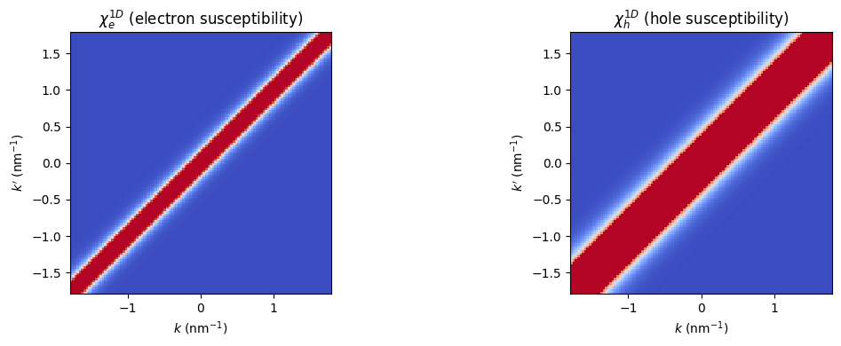
1D Susceptibility Arrays

The Lindhard susceptibility arrays \(\chi^{1D}_e\) and \(\chi^{1D}_h\) are used to compute the dielectric function for screening.

fig, (ax1, ax2) = plt.subplots(1, 2, figsize=(12, 4))

ax1.pcolormesh(k_nm, k_nm, np.real(cm.Chi1De), shading='auto', cmap='coolwarm')
ax1.set_xlabel('$k$ (nm$^{-1}$)')
ax1.set_ylabel("$k'$ (nm$^{-1}$)")
ax1.set_title('$\\chi^{1D}_e$ (electron susceptibility)')
ax1.set_aspect('equal')

ax2.pcolormesh(k_nm, k_nm, np.real(cm.Chi1Dh), shading='auto', cmap='coolwarm')
ax2.set_xlabel('$k$ (nm$^{-1}$)')
ax2.set_ylabel("$k'$ (nm$^{-1}$)")
ax2.set_title('$\\chi^{1D}_h$ (hole susceptibility)')
ax2.set_aspect('equal')

plt.tight_layout()
plt.show()

---

References

1. J. R. Gulley and D. Huang, Opt. Express 27, 17154-17185 (2019). – Coulomb interactions and self-consistent SBE framework.