Architecture: How the SBE Solver Works
Theory
The Semiconductor Bloch Equations (SBEs) are coupled differential equations for the quantum coherence of electrons and holes in a semiconductor under optical excitation. They extend the optical Bloch equations to include many-body Coulomb interactions, carrier-carrier scattering, and phonon effects.
The Three Coupled Equations
1. Electron-Hole Coherence (Interband Polarization):
where \(p_{k_e,k_h}\) is the electron-hole coherence matrix (interband polarization).
2. Electron-Electron Coherence:
Diagonal elements \(C_{k,k} = n_e(k)\) are electron occupation numbers.
3. Hole-Hole Coherence:
Diagonal elements \(D_{k,k} = n_h(k)\) are hole occupation numbers.
Hamiltonian Construction
The effective Hamiltonians include single-particle energies, dipole-field coupling, and screened Coulomb interactions:
Time Evolution
The SBEs use a leapfrog integration scheme with reshuffling for stability:
Leapfrog step: \(X_3 = X_1 + \frac{dX}{dt} \cdot 2\Delta t\) (2nd order accurate)
Reshuffling: \(X_2 = \frac{X_1 + X_3}{2}\) (converts to stable 1st order)
Module Integration
The SBEs module is the central orchestrator. InitializeSBE sets up all
subsystems, and QWCalculator coordinates them at each time step.
Initialization flow:
InitializeSBEreads parameter files (qw.params,mb.params)Calculates material constants and momentum/spatial grids
Initializes subsystems based on flags:
Always:
InitializeQWOptics,InitializeCoulomb,InitializeDephasingIf
Phonon=1:InitializePhononsIf
DCTrans=1:InitializeDCIf
Recomb=1:InitializeEmission
Time evolution flow (each call to QWCalculator):
Prop2QW: Convert propagation fields to QW momentum spaceSBECalculator: Solve SBEs using all initialized modulesQWPolarization3/QWRho5: Calculate polarization and charge densityQW2Prop: Convert QW fields back to propagation space
Parameter Reference
Quantum Wire Parameters (params/qw.params)
Line |
Parameter |
Units |
Description |
Typical Values |
|---|---|---|---|---|
1 |
L |
m |
Wire length |
50-500 nm |
2 |
Delta0 |
m |
Wire thickness (z) |
3-10 nm |
3 |
gap |
eV |
Band gap energy |
GaAs: 1.42-1.5 |
4 |
me |
m\(_0\) |
Electron effective mass |
GaAs: 0.067 |
5 |
mh |
m\(_0\) |
Hole effective mass |
GaAs: 0.45 (heavy) |
6 |
HO |
eV |
Energy level separation |
0.05-0.2 |
7 |
gam_e |
Hz |
Electron dephasing rate |
0.1-10 THz |
8 |
gam_h |
Hz |
Hole dephasing rate |
0.1-10 THz |
9 |
gam_eh |
Hz |
Interband dephasing |
(gam_e + gam_h)/2 |
10 |
epsr |
- |
Relative permittivity |
GaAs: 12-13, AlAs: 9.1 |
11 |
Oph |
eV |
LO phonon energy |
GaAs: 0.036 |
12 |
Gph |
eV |
Phonon damping |
0.001-0.005 |
13 |
Edc |
V/m |
DC electric field |
0 (transport studies) |
14 |
jmax |
- |
Output interval (steps) |
10-1000 |
15 |
ntmax |
- |
Backup interval (steps) |
1000-50000 |
Many-Body Physics Flags (params/mb.params)
Line |
Flag |
Description |
When to Enable |
|---|---|---|---|
1 |
Optics |
Light-matter coupling |
Always (required for optical response) |
2 |
Excitons |
Excitonic correlations |
Exciton physics, bound states |
3 |
EHs |
Carrier-carrier scattering |
Many-body collisions, thermalization |
4 |
Screened |
Screened Coulomb |
Realistic screening (with Excitons) |
5 |
Phonon |
Phonon scattering |
Temperature effects, energy relaxation |
6 |
DCTrans |
DC transport |
Drift/diffusion studies |
7 |
LF |
Longitudinal field |
Plasmon effects, screening dynamics |
8 |
FreePot |
Free potential |
Carrier-induced potential |
9 |
DiagDph |
Diagonal dephasing |
Momentum-dependent dephasing rates |
10 |
OffDiagDph |
Off-diagonal dephasing |
Correlation effects in scattering |
11 |
Recomb |
Spontaneous recombination |
Radiative decay, PL studies |
12 |
PLSpec |
PL spectrum calculation |
Photoluminescence output |
13 |
ignorewire |
Single-wire mode |
Skip inter-wire coupling |
14 |
Xqwparams |
Write chi params |
Output susceptibility files |
15 |
LorentzDelta |
Lorentzian delta |
Numerical broadening method |
Common physics combinations:
Optical Bloch (OBE):
Optics=1, all others0Excitons only:
Optics=1, Excitons=1, Screened=1, DiagDph=1Full many-body:
Optics=1, Excitons=1, EHs=1, Screened=1, DiagDph=1Temperature effects: Add
Phonon=1to aboveTransport: Add
DCTrans=1, LF=1for drift and plasmon effects
1D-to-3D Coupling: SHO Gate Functions
The SBE solver operates in 1D momentum space along the wire axis. But the full simulation couples to a 3D Maxwell PSTD propagator. The bridge between these two worlds uses Simple Harmonic Oscillator (SHO) wavefunctions as spatial gate functions.
Transverse Confinement
The HO parameter in qw.params (100 meV for GaAs) sets the transverse
confinement energy. From this, the code computes inverse confinement lengths:
These define Gaussian envelope functions – the ground-state SHO wavefunctions that describe how the electron and hole probability densities decay in the transverse (y, z) directions away from the wire axis.
Derived Quantities
Electron-hole overlap integral: \(\text{ehint} = \sqrt{2\alpha_e\alpha_h / (\alpha_e^2 + \alpha_h^2)}\) – measures spatial overlap between electron and hole wavefunctions. Closer to 1 means stronger excitonic effects.
Wire cross-section area: \(A = \sqrt{2\pi} \cdot \Delta_0 / \sqrt{\alpha_e^2 + \alpha_h^2}\) – effective transverse area for current and field calculations.
Critical momentum: \(q_c = 2\alpha_e\alpha_h / (\alpha_e + \alpha_h)\) – characteristic momentum scale for Coulomb interactions.
3D Field Placement
When coupling to the Maxwell propagator, the 1D polarization \(\mathbf{P}(x)\)
from the SBE solver is embedded into 3D space using separable Gaussian gates
(from params/qwarray.params):
where \(g_y(y) = \exp\!\left[-(y - y_0)^2 / (2 a_y^2)\right]\) and similarly for \(g_z\).
The gate widths \(a_y\), \(a_z\) are set in qwarray.params (typically 5 nm for GaAs).
This means quantum wires are not mathematical lines – they have real 3D
cross-sections with quantum mechanical confinement profiles. The same SHO
wavefunctions enter the Coulomb interaction integrals in coulomb.py, where
the transverse overlap determines the effective 1D Coulomb potential.
THz Emission from Current Surge
When an ultrashort laser pulse excites carriers in the quantum wire, the rapidly changing polarization acts as a current source:
This polarization current surge emits electromagnetic radiation at terahertz (THz) frequencies – the characteristic timescale of carrier dynamics (femtoseconds to picoseconds corresponds to 0.1-10 THz).
The code computes this current in rhoPJ.py via finite differences:
\(J_x = (P_x^{new} - P_x^{old}) / \Delta t\). An additional free current
component from charge density continuity (\(\mathbf{J}_{free} = -\int \partial\rho/\partial t \, dx\))
contributes to the total THz emission.
THz emission spectroscopy is a major experimental technique for probing
ultrafast carrier dynamics in semiconductors. The infrastructure for tracking
THz fields exists in the codebase (ETHz.t.dat output), with full THz
field analysis planned for future propagator examples.
Inspect an Initialized Solver
Let’s initialize the solver and inspect what was set up.
import os
import numpy as np
import matplotlib.pyplot as plt

from pulsesuite.PSTD3D.SBEs import InitializeSBE, QWCalculator
from pulsesuite.PSTD3D import SBEs as SBEs_module
from pulsesuite.PSTD3D.typespace import GetKArray, GetSpaceArray

# Ensure output directories exist
for d in ['dataQW/Wire/C', 'dataQW/Wire/D', 'dataQW/Wire/Ee',
          'dataQW/Wire/Eh', 'dataQW/Wire/P', 'dataQW/Wire/Win',
          'dataQW/Wire/Wout', 'dataQW/Wire/Xqw', 'dataQW/Wire/info',
          'dataQW/Wire/ne', 'dataQW/Wire/nh', 'output']:
    os.makedirs(d, exist_ok=True)

Nr = 50
drr = 10e-9
rr = GetSpaceArray(Nr, (Nr - 1) * drr)
qrr = GetKArray(Nr, Nr * drr)

InitializeSBE(qrr, rr, 0.0, 1e7, 800e-9, 2, True)
solver = SBEs_module._default_solver

print("=== Grid ===")
print(f"  Nk (momentum points): {solver.Nk}")
print(f"  Nr (QW spatial points): {solver.Nr}")

print("\n=== Material (from qw.params) ===")
print(f"  Band gap: {solver.gap / 1.6e-19:.3f} eV")
print(f"  Electron mass: {solver.me / 9.109e-31:.4f} m0")
print(f"  Hole mass: {solver.mh / 9.109e-31:.4f} m0")

print("\n=== Derived Constants ===")
print(f"  Dipole moment: {solver.dcv:.3e} C*m")
print(f"  Wire cross-section: {solver.area:.3e} m^2")

print("\n=== Physics Flags (from mb.params) ===")
flags = ['Optics', 'Excitons', 'EHs', 'Screened', 'Phonon',
         'DCTrans', 'LF', 'DiagDph', 'OffDiagDph', 'Recomb']
for flag in flags:
    val = getattr(solver, flag)
    status = "ON" if val else "OFF"
    print(f"  {flag:15s}: {status}")
dcv / e0 = 3.3538811268940077e-10
alphae = 303090660.34386384, alphah = 768475083.4742767
1/qc = 2.3003106022655407e-09, sqrt(2) / sqrt(alphae² + alphah²) = 1.7119449377756965e-09
ehint = 0.8262109841666643
Wire Radius = 2.3003106022655407e-09
Wire sqrt(area) = 3.8950888292173374e-09
Wire Thickness = 5e-09
Calculating Coulomb Arrays
  Progress: 0/230 (0.0%)
Vint: Using JIT-compiled version
  Progress: 10/230 (4.3%)
  Progress: 20/230 (8.7%)
  Progress: 30/230 (13.0%)
  Progress: 40/230 (17.4%)
  Progress: 50/230 (21.7%)
  Progress: 60/230 (26.1%)
  Progress: 70/230 (30.4%)
  Progress: 80/230 (34.8%)
  Progress: 90/230 (39.1%)
  Progress: 100/230 (43.5%)
  Progress: 110/230 (47.8%)
  Progress: 120/230 (52.2%)
  Progress: 130/230 (56.5%)
  Progress: 140/230 (60.9%)
  Progress: 150/230 (65.2%)
  Progress: 160/230 (69.6%)
  Progress: 170/230 (73.9%)
  Progress: 180/230 (78.3%)
  Progress: 190/230 (82.6%)
  Progress: 200/230 (87.0%)
  Progress: 210/230 (91.3%)
  Progress: 220/230 (95.7%)
Finished Calculating Unscreened Coulomb Arrays
Quantum Wire Linear Chi = (-0.13219666733079763+0.14243061062572296j)
InitializeSBE?
=== Grid ===
  Nk (momentum points): 114
  Nr (QW spatial points): 230

=== Material (from qw.params) ===
  Band gap: 1.502 eV
  Electron mass: 0.0700 m0
  Hole mass: 0.4500 m0

=== Derived Constants ===
  Dipole moment: 5.374e-29 C*m
  Wire cross-section: 1.517e-17 m^2

=== Physics Flags (from mb.params) ===
  Optics         : ON
  Excitons       : ON
  EHs            : ON
  Screened       : ON
  Phonon         : ON
  DCTrans        : ON
  LF             : ON
  DiagDph        : ON
  OffDiagDph     : ON
  Recomb         : ON
Energy Bands
After initialization, the solver has computed the electron and hole energy bands \(E_e(k)\) and \(E_h(k)\) on the momentum grid.
fig, ax = plt.subplots(figsize=(8, 5))

k_nm = solver.kr * 1e-9  # Convert to 1/nm
Ee_eV = solver.Ee * 6.242e18  # Convert J to eV
Eh_eV = solver.Eh * 6.242e18

ax.plot(k_nm, Ee_eV, 'b-', linewidth=2, label='Electrons $E_e(k)$')
ax.plot(k_nm, -Eh_eV, 'r-', linewidth=2, label='Holes $-E_h(k)$')
ax.axhline(0, color='gray', linewidth=0.5, linestyle='--')

ax.set_xlabel('Momentum $k$ (nm$^{-1}$)')
ax.set_ylabel('Energy (eV)')
ax.set_title('Quantum Wire Energy Bands')
ax.legend()
plt.tight_layout()
plt.show()

print(f"Momentum grid: {solver.Nk} points from "
      f"{solver.kr.min()*1e-9:.2f} to {solver.kr.max()*1e-9:.2f} nm^-1")
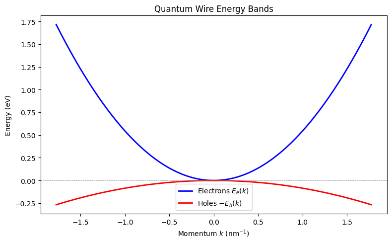
Momentum grid: 114 points from -1.77 to 1.77 nm^-1
Initial Carrier Distributions
The carriers start in thermal equilibrium (Fermi-Dirac at 77 K). The diagonal of the electron coherence matrix \(C_{k,k} = n_e(k)\) gives the electron occupation.
# Extract initial carrier distributions (diagonal of CC2 for wire 1)
ne = np.real(np.diag(solver.CC2[:, :, 0]))  # Electron occupation
nh = np.real(np.diag(solver.DD2[:, :, 0]))  # Hole occupation

fig, ax = plt.subplots(figsize=(8, 4))
ax.plot(k_nm, ne, 'b-', linewidth=2, label='$n_e(k)$')
ax.plot(k_nm, nh, 'r-', linewidth=2, label='$n_h(k)$')

ax.set_xlabel('Momentum $k$ (nm$^{-1}$)')
ax.set_ylabel('Occupation')
ax.set_title('Initial Carrier Distributions (T = 77 K)')
ax.legend()
plt.tight_layout()
plt.show()

print(f"Total electron density: {ne.sum():.4e}")
print(f"Total hole density: {nh.sum():.4e}")
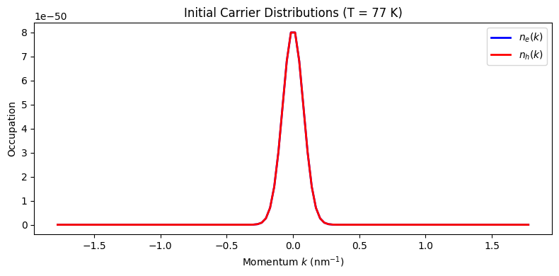
Total electron density: 5.0780e-49
Total hole density: 5.0780e-49
References
J. R. Gulley and D. Huang, “Self-consistent quantum-kinetic theory for interplay between pulsed-laser excitation and nonlinear carrier transport in a quantum-wire array,” Opt. Express 27, 17154-17185 (2019).
J. R. Gulley and D. Huang, “Ultrafast transverse and longitudinal response of laser-excited quantum wires,” Opt. Express 30(6), 9348-9359 (2022).
M. Lindberg and S. W. Koch, “Effective Bloch equations for semiconductors,” Phys. Rev. B 38, 3342 (1988).