Deep Dive: Phonon Interactions
Theory
Carriers in the quantum wire interact with longitudinal optical (LO) phonons through the Frohlich interaction. This provides the dominant energy relaxation mechanism at finite temperature.
Phonon Absorption and Emission
Carriers can absorb or emit LO phonons:
Absorption: \(\Gamma_{abs}(k, k') \propto N_0 \cdot \delta(E_k - E_{k'} - \hbar\omega_{ph})\)
Emission: \(\Gamma_{em}(k, k') \propto (N_0 + 1) \cdot \delta(E_k - E_{k'} + \hbar\omega_{ph})\)
where \(N_0 = [\exp(\hbar\omega_{ph} / k_B T) - 1]^{-1}\) is the Bose-Einstein distribution for thermal phonons.
Phonon Interaction Matrix
The matrix elements use Lorentzian broadening of the energy-conserving delta function:
where \(\omega_{ph}\) is the phonon frequency and \(\gamma_{ph}\) is the phonon damping rate.
Many-Body Phonon Scattering
The many-body scattering rates include Pauli blocking:
Assumptions and Parameter Choices
Important
The parameters below come from params/qw.params and are read automatically
by InitializeSBE. They correspond to a GaAs quantum wire in an AlAs host.
LO Phonon energy: 36 meV – the GaAs longitudinal optical phonon
Phonon damping: 3 meV – typical inverse phonon lifetime
Host dielectric constants: \(\epsilon_0 = 10.0\), \(\epsilon_\infty = 8.2\) (AlAs)
Temperature: 77 K (liquid nitrogen) – common experimental condition
Effective masses: \(m_e = 0.07 \, m_0\), \(m_h = 0.45 \, m_0\) (GaAs)
Warning
The phonon module currently uses module-level variables for temperature
(phonons._Temp = 77.0). Changing temperature requires re-initialization.
Initialize and Inspect
import os
import numpy as np
import matplotlib.pyplot as plt
from scipy.constants import hbar as hbar_SI, k as kB_SI

from pulsesuite.PSTD3D.SBEs import InitializeSBE
from pulsesuite.PSTD3D import SBEs as SBEs_module
from pulsesuite.PSTD3D import phonons
from pulsesuite.PSTD3D.typespace import GetKArray, GetSpaceArray

# Ensure output directories exist
for d in ['dataQW/Wire/C', 'dataQW/Wire/D', 'dataQW/Wire/Ee',
          'dataQW/Wire/Eh', 'dataQW/Wire/P', 'dataQW/Wire/Win',
          'dataQW/Wire/Wout', 'dataQW/Wire/Xqw', 'dataQW/Wire/info',
          'dataQW/Wire/ne', 'dataQW/Wire/nh', 'output']:
    os.makedirs(d, exist_ok=True)

Nr = 50
drr = 10e-9
rr = GetSpaceArray(Nr, (Nr - 1) * drr)
qrr = GetKArray(Nr, Nr * drr)

InitializeSBE(qrr, rr, 0.0, 1e7, 800e-9, 2, True)
solver = SBEs_module._default_solver

print(f"Temperature: {phonons._Temp} K")
print(f"Bose occupation N0: {phonons._NO:.4f}")
print(f"Phonon energy: {solver.Oph * hbar_SI / 1.6e-19 * 1e3:.1f} meV")
print(f"Phonon damping: {solver.Gph * hbar_SI / 1.6e-19 * 1e3:.1f} meV")
print(f"EP matrix shape: {phonons._EP.shape}")
dcv / e0 = 3.3538811268940077e-10
alphae = 303090660.34386384, alphah = 768475083.4742767
1/qc = 2.3003106022655407e-09, sqrt(2) / sqrt(alphae² + alphah²) = 1.7119449377756965e-09
ehint = 0.8262109841666643
Wire Radius = 2.3003106022655407e-09
Wire sqrt(area) = 3.8950888292173374e-09
Wire Thickness = 5e-09
Calculating Coulomb Arrays
  Progress: 0/230 (0.0%)
Vint: Using JIT-compiled version
  Progress: 10/230 (4.3%)
  Progress: 20/230 (8.7%)
  Progress: 30/230 (13.0%)
  Progress: 40/230 (17.4%)
  Progress: 50/230 (21.7%)
  Progress: 60/230 (26.1%)
  Progress: 70/230 (30.4%)
  Progress: 80/230 (34.8%)
  Progress: 90/230 (39.1%)
  Progress: 100/230 (43.5%)
  Progress: 110/230 (47.8%)
  Progress: 120/230 (52.2%)
  Progress: 130/230 (56.5%)
  Progress: 140/230 (60.9%)
  Progress: 150/230 (65.2%)
  Progress: 160/230 (69.6%)
  Progress: 170/230 (73.9%)
  Progress: 180/230 (78.3%)
  Progress: 190/230 (82.6%)
  Progress: 200/230 (87.0%)
  Progress: 210/230 (91.3%)
  Progress: 220/230 (95.7%)
Finished Calculating Unscreened Coulomb Arrays
Quantum Wire Linear Chi = (-0.13219666733079763+0.14243061062572296j)
InitializeSBE?
Temperature: 77.0 K
Bose occupation N0: 0.0044
Phonon energy: 36.0 meV
Phonon damping: 3.0 meV
EP matrix shape: (114, 114)
Phonon Interaction Matrices
The electron phonon matrix \(EP(k, k')\) and hole phonon matrix \(HP(k, k')\) show peaks where the energy difference \(E_k - E_{k'}\) matches the phonon energy \(\pm\hbar\omega_{ph}\).
fig, (ax1, ax2) = plt.subplots(1, 2, figsize=(12, 5))

k_nm = solver.kr * 1e-9

im1 = ax1.pcolormesh(k_nm, k_nm, phonons._EP, shading='auto', cmap='hot')
ax1.set_xlabel('$k$ (nm$^{-1}$)')
ax1.set_ylabel("$k'$ (nm$^{-1}$)")
ax1.set_title('Electron-Phonon $EP(k, k\')$')
ax1.set_aspect('equal')
plt.colorbar(im1, ax=ax1)

im2 = ax2.pcolormesh(k_nm, k_nm, phonons._HP, shading='auto', cmap='hot')
ax2.set_xlabel('$k$ (nm$^{-1}$)')
ax2.set_ylabel("$k'$ (nm$^{-1}$)")
ax2.set_title('Hole-Phonon $HP(k, k\')$')
ax2.set_aspect('equal')
plt.colorbar(im2, ax=ax2)

plt.suptitle(f'Phonon Interaction Matrices (T = {phonons._Temp:.0f} K)', y=1.02)
plt.tight_layout()
plt.show()

print(f"EP range: {phonons._EP.min():.3e} to {phonons._EP.max():.3e}")
print(f"HP range: {phonons._HP.min():.3e} to {phonons._HP.max():.3e}")
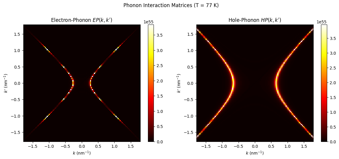
EP range: 0.000e+00 to 3.844e+55
HP range: 0.000e+00 to 3.961e+55
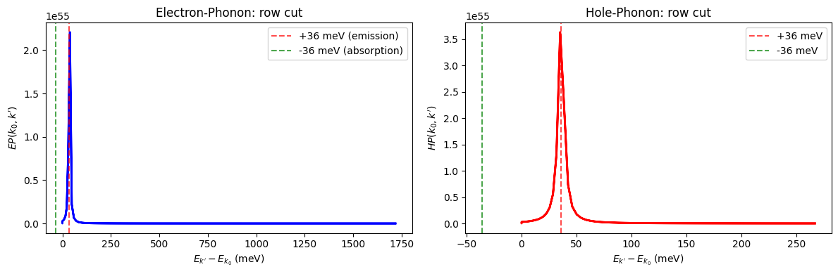
Energy-Difference Structure
A row cut of \(EP\) at fixed \(k_0\) reveals the Lorentzian peaks at \(E_{k'} = E_{k_0} \pm \hbar\omega_{ph}\) corresponding to phonon emission and absorption.
mid_k = solver.Nk // 2
eV = 1.6e-19

fig, (ax1, ax2) = plt.subplots(1, 2, figsize=(12, 4))

# EP row cut
dE_eV = (solver.Ee - solver.Ee[mid_k]) / eV * 1e3  # meV
ax1.plot(dE_eV, phonons._EP[mid_k, :], 'b-', linewidth=2)
ax1.axvline(36, color='red', linestyle='--', alpha=0.7, label='+36 meV (emission)')
ax1.axvline(-36, color='green', linestyle='--', alpha=0.7, label='-36 meV (absorption)')
ax1.set_xlabel("$E_{k'} - E_{k_0}$ (meV)")
ax1.set_ylabel('$EP(k_0, k\')$')
ax1.set_title('Electron-Phonon: row cut')
ax1.legend()

# HP row cut
dE_eV_h = (solver.Eh - solver.Eh[mid_k]) / eV * 1e3
ax2.plot(dE_eV_h, phonons._HP[mid_k, :], 'r-', linewidth=2)
ax2.axvline(36, color='red', linestyle='--', alpha=0.7, label='+36 meV')
ax2.axvline(-36, color='green', linestyle='--', alpha=0.7, label='-36 meV')
ax2.set_xlabel("$E_{k'} - E_{k_0}$ (meV)")
ax2.set_ylabel('$HP(k_0, k\')$')
ax2.set_title('Hole-Phonon: row cut')
ax2.legend()

plt.tight_layout()
plt.show()
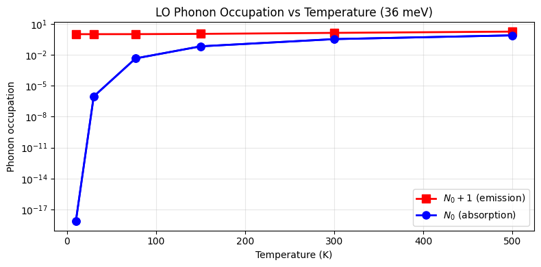
Temperature Dependence
The Bose-Einstein distribution \(N_0(T)\) controls the balance between phonon absorption and emission. At low temperatures, emission dominates.
T_range = np.array([10, 30, 77, 150, 300, 500])
Oph_eV = 36e-3  # phonon energy in eV
Oph_J = Oph_eV * eV

N0_vals = 1.0 / (np.exp(Oph_J / (kB_SI * T_range)) - 1.0)

fig, ax = plt.subplots(figsize=(8, 4))
ax.semilogy(T_range, N0_vals, 'bo-', markersize=8, linewidth=2)
ax.semilogy(T_range, N0_vals + 1, 'rs-', markersize=8, linewidth=2, label='$N_0 + 1$ (emission)')
ax.semilogy(T_range, N0_vals, 'bo-', markersize=8, linewidth=2, label='$N_0$ (absorption)')

ax.set_xlabel('Temperature (K)')
ax.set_ylabel('Phonon occupation')
ax.set_title('LO Phonon Occupation vs Temperature (36 meV)')
ax.legend()
ax.grid(True, alpha=0.3)
plt.tight_layout()
plt.show()

print("Temperature | N0 (absorption) | N0+1 (emission) | Emission/Absorption ratio")
print("-" * 75)
for T, N0 in zip(T_range, N0_vals):
    ratio = (N0 + 1) / N0 if N0 > 0 else float('inf')
    print(f"  {T:4.0f} K    |    {N0:.4e}    |    {N0+1:.4f}       |    {ratio:.2f}")
Temperature | N0 (absorption) | N0+1 (emission) | Emission/Absorption ratio
---------------------------------------------------------------------------
    10 K    |    7.6111e-19    |    1.0000       |    1313871994298542080.00
    30 K    |    9.1303e-07    |    1.0000       |    1095261.16
    77 K    |    4.4552e-03    |    1.0045       |    225.45
   150 K    |    6.6050e-02    |    1.0661       |    16.14
   300 K    |    3.3140e-01    |    1.3314       |    4.02
   500 K    |    7.6722e-01    |    1.7672       |    2.30
References
J. R. Gulley and D. Huang, Opt. Express 27, 17154-17185 (2019). – Phonon scattering within the self-consistent SBE framework.