Deep Dive: Quantum Wire Optics

Theory

The qwoptics module handles the interface between the classical electromagnetic field (living on a real-space propagation grid) and the quantum mechanical calculations (living in momentum space on the wire).

Prop2QW and QW2Prop Workflow

Propagation to QW (Prop2QW):

1. Interpolate Maxwell fields from propagation grid to QW grid

2. Apply the quantum wire window function to confine fields to the wire region

3. FFT to convert from real space to momentum space

QW to Propagation (QW2Prop):

1. Inverse FFT to convert from momentum space to real space

2. Interpolate QW fields back to propagation grid

3. Normalize charge densities for consistency

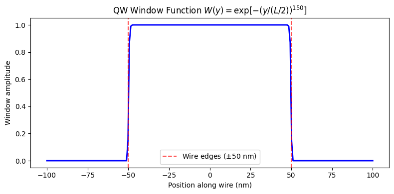
QW Window Function

The window function confines the fields to the wire length \(L\):

\[ W(y) = \exp\!\left[-\left(\frac{y}{L/2}\right)^{150}\right] \]

The exponent 150 gives an extremely sharp cutoff – essentially a rectangular window with smooth edges to avoid Gibbs ringing in the FFT.

Linear Susceptibility

The linear optical susceptibility of the quantum wire is:

\[ \chi^{(1)}(\omega) = \frac{4 |d_{cv}|^2}{\hbar \, A_{wire}} \sum_k \left[ \frac{1}{E_e(k) + E_h(k) - i\hbar\gamma_{eh} - \hbar\omega} + \frac{1}{E_e(k) + E_h(k) + i\hbar\gamma_{eh} + \hbar\omega} \right] \Delta k \]

where \(d_{cv}\) is the dipole matrix element, \(A_{wire}\) is the wire cross-section, and \(\gamma_{eh}\) is the interband dephasing rate.

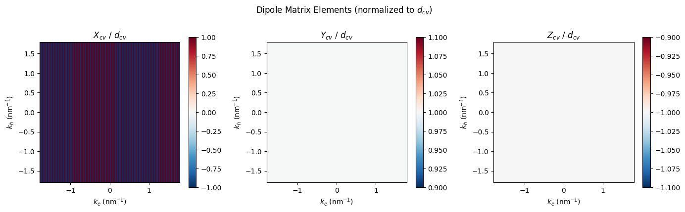
Dipole Matrix Elements

The dipole coupling between valence and conduction bands has different symmetry for each polarization direction:

• \(X_{cv}(k_e, k_h) = d_{cv} \cdot (-1)^{k_h}\) (parity-dependent)

• \(Y_{cv}(k_e, k_h) = d_{cv}\) (uniform)

• \(Z_{cv}(k_e, k_h) = -d_{cv}\) (opposite sign)

---

Initialize and Inspect

import os
import numpy as np
import matplotlib.pyplot as plt
from scipy.constants import c as c0_SI, hbar as hbar_SI

from pulsesuite.PSTD3D.SBEs import InitializeSBE
from pulsesuite.PSTD3D import SBEs as SBEs_module
from pulsesuite.PSTD3D.qwoptics import QWChi1
from pulsesuite.PSTD3D.typespace import GetKArray, GetSpaceArray

# Ensure output directories exist
for d in ['dataQW/Wire/C', 'dataQW/Wire/D', 'dataQW/Wire/Ee',
          'dataQW/Wire/Eh', 'dataQW/Wire/P', 'dataQW/Wire/Win',
          'dataQW/Wire/Wout', 'dataQW/Wire/Xqw', 'dataQW/Wire/info',
          'dataQW/Wire/ne', 'dataQW/Wire/nh', 'output']:
    os.makedirs(d, exist_ok=True)

Nr = 50
drr = 10e-9
rr = GetSpaceArray(Nr, (Nr - 1) * drr)
qrr = GetKArray(Nr, Nr * drr)

InitializeSBE(qrr, rr, 0.0, 1e7, 800e-9, 2, True)
solver = SBEs_module._default_solver
qw = solver.qw  # QWOptics instance

print(f"QW Optics initialized: Nr_qw={solver.Nr}, Nk={solver.Nk}")
print(f"Wire length L: {solver.L*1e9:.0f} nm")
print(f"Dipole moment dcv: {solver.dcv:.3e} C*m")
print(f"Wire cross-section: {solver.area:.3e} m^2")

dcv / e0 = 3.3538811268940077e-10
alphae = 303090660.34386384, alphah = 768475083.4742767
1/qc = 2.3003106022655407e-09, sqrt(2) / sqrt(alphae² + alphah²) = 1.7119449377756965e-09
ehint = 0.8262109841666643
Wire Radius = 2.3003106022655407e-09
Wire sqrt(area) = 3.8950888292173374e-09
Wire Thickness = 5e-09

Calculating Coulomb Arrays
  Progress: 0/230 (0.0%)
Vint: Using JIT-compiled version
  Progress: 10/230 (4.3%)
  Progress: 20/230 (8.7%)
  Progress: 30/230 (13.0%)
  Progress: 40/230 (17.4%)
  Progress: 50/230 (21.7%)
  Progress: 60/230 (26.1%)
  Progress: 70/230 (30.4%)
  Progress: 80/230 (34.8%)
  Progress: 90/230 (39.1%)
  Progress: 100/230 (43.5%)
  Progress: 110/230 (47.8%)
  Progress: 120/230 (52.2%)
  Progress: 130/230 (56.5%)
  Progress: 140/230 (60.9%)
  Progress: 150/230 (65.2%)
  Progress: 160/230 (69.6%)
  Progress: 170/230 (73.9%)
  Progress: 180/230 (78.3%)
  Progress: 190/230 (82.6%)
  Progress: 200/230 (87.0%)
  Progress: 210/230 (91.3%)
  Progress: 220/230 (95.7%)
Finished Calculating Unscreened Coulomb Arrays

Quantum Wire Linear Chi = (-0.13219666733079763+0.14243061062572296j)

InitializeSBE?
QW Optics initialized: Nr_qw=230, Nk=114
Wire length L: 100 nm
Dipole moment dcv: 5.374e-29 C*m
Wire cross-section: 1.517e-17 m^2

QW Window Function

The super-Gaussian window function that confines fields to the wire region. This ensures fields outside the wire don’t contribute to the quantum calculation.

fig, ax = plt.subplots(figsize=(8, 4))

y_grid = solver.r  # Real-space grid on QW
y_nm = y_grid * 1e9

ax.plot(y_nm, qw._QWWindow, 'b-', linewidth=2)
ax.axvline(-solver.L/2 * 1e9, color='red', linestyle='--', alpha=0.7, label=f'Wire edges ($\\pm${solver.L*1e9/2:.0f} nm)')
ax.axvline(solver.L/2 * 1e9, color='red', linestyle='--', alpha=0.7)

ax.set_xlabel('Position along wire (nm)')
ax.set_ylabel('Window amplitude')
ax.set_title('QW Window Function $W(y) = \\exp[-(y/(L/2))^{150}]$')
ax.legend()
plt.tight_layout()
plt.show()

Dipole Matrix Elements

The three polarization-dependent dipole matrices \(X_{cv}\), \(Y_{cv}\), \(Z_{cv}\) couple the valence and conduction bands.

fig, axes = plt.subplots(1, 3, figsize=(14, 4))

k_nm = solver.kr * 1e-9

for ax, M, title in zip(axes,
                         [qw._Xcv0, qw._Ycv0, qw._Zcv0],
                         ['$X_{cv}$', '$Y_{cv}$', '$Z_{cv}$']):
    im = ax.pcolormesh(k_nm, k_nm, np.real(M) / solver.dcv,
                        shading='auto', cmap='RdBu_r')
    ax.set_xlabel('$k_e$ (nm$^{-1}$)')
    ax.set_ylabel('$k_h$ (nm$^{-1}$)')
    ax.set_title(f'{title} / $d_{{cv}}$')
    ax.set_aspect('equal')
    plt.colorbar(im, ax=ax)

plt.suptitle('Dipole Matrix Elements (normalized to $d_{cv}$)', y=1.02)
plt.tight_layout()
plt.show()

Linear Susceptibility Spectrum

Compute \(\chi^{(1)}(\omega)\) over a range of photon energies near the band gap. The imaginary part gives the absorption spectrum, while the real part gives the refractive index change.

eV = 1.6e-19
c0 = c0_SI

# Scan wavelengths from 700 to 900 nm (around band gap at ~1.5 eV = 827 nm)
lam_range = np.linspace(700e-9, 900e-9, 200)
E_photon = 6.626e-34 * c0 / lam_range / eV  # photon energy in eV

dky = solver.kr[1] - solver.kr[0] if solver.Nk > 1 else 1.0

chi1_vals = np.array([
    QWChi1(lam, dky, solver.Ee, solver.Eh, solver.area, solver.gam_eh, solver.dcv)
    for lam in lam_range
])

fig, (ax1, ax2) = plt.subplots(2, 1, figsize=(10, 7), sharex=True)

ax1.plot(E_photon, np.imag(chi1_vals), 'r-', linewidth=2)
ax1.axvline(solver.gap / eV, color='gray', linestyle='--', alpha=0.7,
            label=f'Band gap ({solver.gap/eV:.2f} eV)')
ax1.set_ylabel('Im $\\chi^{(1)}$')
ax1.set_title('Linear Susceptibility of GaAs Quantum Wire')
ax1.legend()

ax2.plot(E_photon, np.real(chi1_vals), 'b-', linewidth=2)
ax2.axvline(solver.gap / eV, color='gray', linestyle='--', alpha=0.7)
ax2.set_xlabel('Photon Energy (eV)')
ax2.set_ylabel('Re $\\chi^{(1)}$')

plt.tight_layout()
plt.show()

print(f"Band gap: {solver.gap/eV:.3f} eV ({6.626e-34*c0/(solver.gap)*1e9:.0f} nm)")
print(f"Peak absorption at: {E_photon[np.argmax(np.imag(chi1_vals))]:.3f} eV")

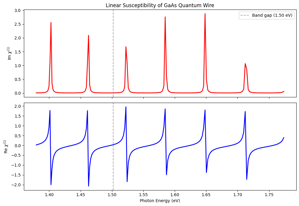
Band gap: 1.502 eV (827 nm)
Peak absorption at: 1.648 eV

---

References

1. J. R. Gulley and D. Huang, Opt. Express 27, 17154-17185 (2019).

2. J. R. Gulley and D. Huang, Opt. Express 30(6), 9348-9359 (2022). – Transverse and longitudinal optical response.